Basic usage

import elpigraph
import numpy as np
import matplotlib.pyplot as plt

# load toy data
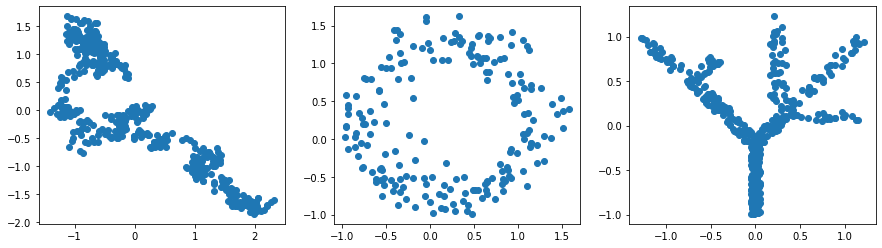
X_curve = np.loadtxt('../data/curve_data.csv',delimiter=',')[:,:2]
X_circle = np.loadtxt('../data/circle_data.csv',delimiter=',')[:,:2]
X_tree = np.loadtxt('../data/tree_data.csv',delimiter=',')[:,:2]

f,axs=plt.subplots(1,3,figsize=(15,4))
axs[0].scatter(*X_curve.T)
axs[1].scatter(*X_circle.T)
axs[2].scatter(*X_tree.T)
plt.show()

Fitting principal graphs

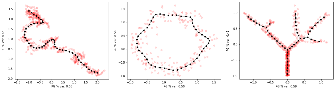
We can fit a principal graph with appropriate topology for each dataset, with specified number of graph nodes

pg_curve = elpigraph.computeElasticPrincipalCurve(X_curve,NumNodes=50)[0]
pg_circle = elpigraph.computeElasticPrincipalCircle(X_circle,NumNodes=50)[0]
pg_tree = elpigraph.computeElasticPrincipalTree(X_tree,NumNodes=50)[0]

# plot graph (NodePositions and Edges) and data
f,axs=plt.subplots(1,3,figsize=(20,5))
axs=axs.flat
elpigraph.plot.PlotPG(X_curve,pg_curve,Do_PCA=False,show_text=False,ax=next(axs))
elpigraph.plot.PlotPG(X_circle,pg_circle,Do_PCA=False,show_text=False,ax=next(axs))
elpigraph.plot.PlotPG(X_tree,pg_tree,Do_PCA=False,show_text=False,ax=next(axs))
plt.show()

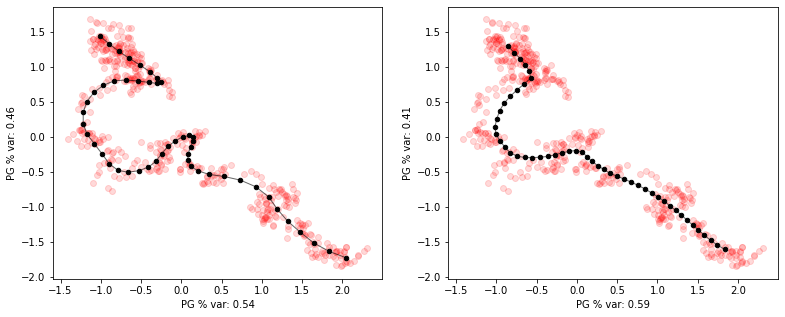
Main parameters to tune are: * NumNodes : the number of nodes of the graph

• Lambda : the attractive strength of edges between nodes (constrains edge lengths)
• Mu : the repulsive strength of a node’s neighboring nodes (constrains angles to be close to harmonic)
• alpha : branching penalty (penalizes number of branches for the principal tree)

# illustrate tuning Lambda
f,axs=plt.subplots(1,2,figsize=(13,5))
axs=axs.flat

pg_curve = elpigraph.computeElasticPrincipalCurve(X_curve,NumNodes=50,Lambda=0.001)[0]
elpigraph.plot.PlotPG(X_curve,pg_curve,Do_PCA=False,show_text=False,ax=next(axs))

pg_curve = elpigraph.computeElasticPrincipalCurve(X_curve,NumNodes=50,Lambda=0.1)[0]
elpigraph.plot.PlotPG(X_curve,pg_curve,Do_PCA=False,show_text=False,ax=next(axs))
plt.show()

# illustrate tuning Lambda
f,axs=plt.subplots(1,2,figsize=(13,5))
axs=axs.flat

# illustrate tuning Mu
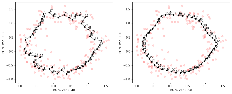
pg_curve = elpigraph.computeElasticPrincipalCircle(X_circle,NumNodes=50,Mu=0.001)[0]
elpigraph.plot.PlotPG(X_circle,pg_curve,Do_PCA=False,ax=next(axs))

pg_curve = elpigraph.computeElasticPrincipalCircle(X_circle,NumNodes=50,Mu=0.2)[0]
elpigraph.plot.PlotPG(X_circle,pg_curve,Do_PCA=False,ax=next(axs))

plt.show()

Projecting and ordering cells along the graph

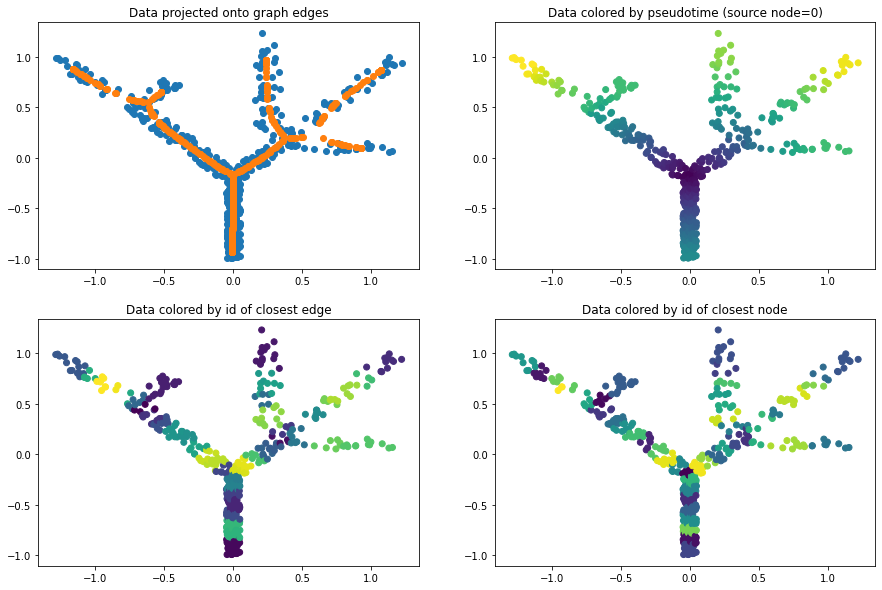
# results are directly stored in pg_tree as a dictionary
source_node = 0
elpigraph.utils.getPseudotime(X_tree,pg_tree,source=source_node,target=None)

dict_proj = pg_tree['projection']
pseudotime = pg_tree['pseudotime']

f, axs = plt.subplots(2,2,figsize=(15,10))
axs = axs.flat
titles = ['Data projected onto graph edges',  f'Data colored by pseudotime (source node={source_node})',
          'Data colored by id of closest edge', 'Data colored by id of closest node']
colors = [None, pseudotime, dict_proj['edge_id'], dict_proj['node_id']]

for i in range(4):
    ax=next(axs)
    ax.scatter(*X_tree.T,c=colors[i])
    if i==0: ax.scatter(*dict_proj['X_projected'].T)
    ax.set_title(titles[i])
plt.show()

Speeding up computations

Computations can be sped up by reducing the number of candidate graphs topologies considered at each step.

This is especially useful for high number of nodes, where number of candidates starts growing fast

%time pg_tree = elpigraph.computeElasticPrincipalTree(X_tree,50)[0]
%time pg_tree = elpigraph.computeElasticPrincipalTree(X_tree,50,MaxNumberOfGraphCandidatesDict={"AddNode2Node":20,"BisectEdge":10,"ShrinkEdge":10})[0]
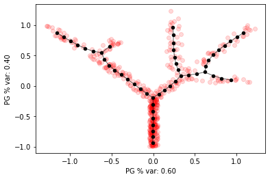
elpigraph.plot.PlotPG(X_tree,pg_tree,Do_PCA=False,show_text=False)

CPU times: user 1min 20s, sys: 1min 7s, total: 2min 27s
Wall time: 12.9 s
CPU times: user 36.6 s, sys: 31.2 s, total: 1min 7s
Wall time: 6.13 s